
This case studies section shows the methods to produce World Grid Squares statistics from point data including geographic information (latitude and longitude). The method to visualize given World Grid Squares statistics by using R is also introduced here with some example codes. The execution environment to use R is required. Rstudio is available as an integrated development environment, so please prepare both the execution and development environment prior to execute following source codes.
How to produce World Grid Square statistics
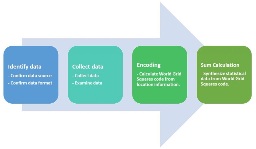
Figure 1: Work Flow to produce World Grid Square statistics
The process to produce World Grid Square statistics can be divided into four phases. To convert point data including geographic information (latitude and longitude) into World Grid Squares statistics, you can calculate World Grid Squares codes according to the information of latitude and longitude in each record. Figure 1 shows the workflow to produce World Grid Squares statistics. The detailed procedure of each phase is described as follows:
1) Data identification:
Firstly, it is required to identify the data source including geographic information and to understand the data format and meaning of the data in the contexts. At that time, making the contract about the usage of data with the original data holder should be taken into account. The range of data usage including secondary usage should be specified in the agreements.
2) Data collection:
After identifying the data source, the data need to be collected repeatedly and converted into a usable format such as csv file, so that the data could be usable at any time in the database. While collecting data, any errors, missing or corrupted data should be checked.
3) Encoding:
From collected data including geographic information (latitude and longitude), you can compute the World Grid Squares codes from geographic information by using open library. The calculated World Grid Square codes can be given to each data record, categorized and labeled which data records are included in given World Grid Square codes.
4) Data aggregation:
Lastly, by using the World Grid Squares given to each data records through encoding, statistics data products can be read out after the operations of summing up and other statistical processing.
The following R language code can be used to produce World Grid Square statistics from points data including geographic information (latitude and longitude). It is assumed that the csv file [20170531.csv] is placed under the same directory as the R source code.

source("http://www.fttsus.jp/worldmesh/R/worldmesh.R")
mydir<-getwd()
infile<- paste0(mydir,"/20170531.csv")
ofile<- paste0(mydir,"/out_mesh3.csv")
a<-read.csv(infile,fileEncoding="UTF-8",header=F)
b<-head(a,100) # attempt to calculate the world grid square statistics by using the first 100 records.
mm<-c() for(i in 1:nrow(b)){ if(nchar(as.character(b[i,]$V13))>4){
      lat0<-unlist(strsplit(x=as.character(b[i,]$V13),split='[NS.]'))
      long0<-unlist(strsplit(x=as.character(b[i,]$V14),split='[WE.]'))
      lat<-as.numeric(lat0[2])+as.numeric(lat0[3])/60+as.numeric(lat0[4])/3600
      long<-as.numeric(long0[2])+as.numeric(long0[3])/60+as.numeric(long0[4])/3600
      wmeshcode <- cal_meshcode(lat,long)
      cat(sprintf("%s,%s,%s,%s,%s,%s,%s\n",wmeshcode,b[i,]$V1,b[i,]$V2,b[i,]$V3,b[i,]$V4,b[i,]$V5,b[i,]$V6))
      mm[i]<-wmeshcode
  }
}
wm<-unique(mm)
cat(file=ofile,sprintf("worldmeshcode,lat0,long0,lat1,long1,cnt\n"),append=F)
for(wmm in wm){
    cnt<-length(mm[mm==wmm&!is.na(mm)])
    res<-meshcode_to_latlong_grid(wmm)
    cat(file=ofile,sprintf("%s,%f,%f,%f,%f,%d\n",wmm,res$lat0,res$long0,res$lat1,res$long1,cnt),append=T)
}
The output resulting from the R source code includes southern longitude, western longitude, northern latitude, eastern latitude and the number of recruitment advertisement. As increasing the number of data records by setting a as more than 100 in head(a, 100), the World Grid Square statistics about job advertisement will be generated from more data records.
[Examples of output codes]
worldmeshcode,lat0,long0,lat1,long1,cnt
2053394526,35.691667,139.700000,35.683333,139.712500,2
2053393586,35.658333,139.700000,35.650000,139.712500,3
2053394601,35.675000,139.762500,35.666667,139.775000,2
2053394577,35.733333,139.712500,35.725000,139.725000,2
2053394611,35.683333,139.762500,35.675000,139.775000,2
2053393578,35.650000,139.725000,35.641667,139.737500,1
2053403039,35.616667,140.112500,35.608333,140.125000,2
2053394578,35.733333,139.725000,35.725000,139.737500,1
2053394507,35.675000,139.712500,35.666667,139.725000,1
2053394579,35.733333,139.737500,35.725000,139.750000,1
2053393566,35.641667,139.700000,35.633333,139.712500,1
2053394528,35.691667,139.725000,35.683333,139.737500,1
2053394672,35.733333,139.775000,35.725000,139.787500,1
2053396249,35.875000,139.362500,35.866667,139.375000,1
2054404345,36.375000,140.437500,36.366667,140.450000,1
2053393596,35.666667,139.700000,35.658333,139.712500,2
2053396522,35.858333,139.650000,35.850000,139.662500,1
2053393263,35.641667,139.287500,35.633333,139.300000,1
2053391541,35.458333,139.637500,35.450000,139.650000,1
2053393642,35.625000,139.775000,35.616667,139.787500,2
2053394353,35.716667,139.412500,35.708333,139.425000,1
2054407544,36.625000,140.675000,36.616667,140.687500,1
2053393547,35.625000,139.712500,35.616667,139.725000,1
2053394506,35.675000,139.700000,35.666667,139.712500,1
2053394709,35.675000,139.987500,35.666667,140.000000,1
2053392415,35.516667,139.562500,35.508333,139.575000,1
2053394632,35.700000,139.775000,35.691667,139.787500,9
2053407531,35.950000,140.637500,35.941667,140.650000,1
2053394576,35.733333,139.700000,35.725000,139.712500,1
2053393548,35.625000,139.725000,35.616667,139.737500,1
2053391530,35.450000,139.625000,35.441667,139.637500,1
2053391459,35.466667,139.612500,35.458333,139.625000,2
2053394435,35.700000,139.562500,35.691667,139.575000,1
2053394652,35.716667,139.775000,35.708333,139.787500,1
2053393394,35.666667,139.425000,35.658333,139.437500,1
2053393691,35.666667,139.762500,35.658333,139.775000,1
2053396463,35.891667,139.537500,35.883333,139.550000,1
2053392345,35.541667,139.437500,35.533333,139.450000,1
2053393559,35.633333,139.737500,35.625000,139.750000,1
2053393390,35.666667,139.375000,35.658333,139.387500,1
2053393330,35.616667,139.375000,35.608333,139.387500,1
2053394504,35.675000,139.675000,35.666667,139.687500,1
2053394612,35.683333,139.775000,35.675000,139.787500,1
2053394446,35.708333,139.575000,35.700000,139.587500,1
2053394543,35.708333,139.662500,35.700000,139.675000,1
How to visualize World Grid Square statistics
Here is the explanation of the method to visualize the World Grid Square statistics by using the leaflet from R library and mapview.
Firstly, please install the libraries of leaflet and mapview to your R execution environment by using the following steps:
install.packages(“leaflet”)
install.packages(“mapview”)
This R source firstly reads the World Grid Square statistics given to each nation and identify the range of drawing from the information of longitudes and latitudes. Then, the png format image data is generated automatically by using mapshop function. Once leaflet including html is generated inside, and then the image is generated by converting the html file into the png image file. To run the R code, PhantomJS is required. PhantomJS can be installed by running
webshot::install shantomjs()
from R command line.
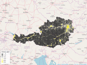
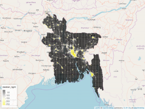
The source code is as follows. By placing the tsv file which is downloadable from the website of the World Grid Squares->Data->NASA night-time light intensity data product and running the R source code, the visualized image data could be generated in png format. Figure 2 shows the examples of the images of Austria, Bangladesh and Taiwan output by using the NASA night-time light intensity data product in 2012. To generate those images, following data are downloaded and used: NASA_AUT_mesh3.tsv, NASA_BGD_mesh3.tsv, and NASA_TWN_mesh3.tsv.
(b) Bangladesh
(c) Taiwan
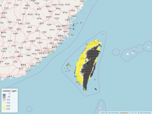
Figure 2: Visualized images of 3rd-level grid square statistics for night-time light intensity (a) Austria, (b) bangladesh, (c) Taiwan
[R Sorce Code(create_iamge_NASA_light.r)]
# This source code needs PhantomJS.
# PhantomJS can be installed by using webshot::install_phantomjs().
library(leaflet)
library(mapview)
#color
cols<-colorRamp(c("#000000","white","#faf500"))
pal<-colorNumeric(palette=cols, domain=(0:255))

#homedir<-"~/JST/assistant/H28/Jin/NASA_light"
homedir <- getwd()
targetdir<-dir(path=homedir,pattern="tsv")
for(d in targetdir){
  tt<-unlist(strsplit(d,"[/.]"))
  if(tt[2]=="tsv"){
    infile<-d
    ofile<-paste0(tt[1],".png")
    t<-read.csv(paste0(homedir,"/",infile), sep="\t", header=TRUE)
    longmax<-max(t$long0)
    longmin<-min(t$long1)
    latmax<-max(t$lat0)
    latmin<-min(t$lat1) if(((longmax-longmin)/200*3600/45)>1){
      dlong<-(longmax-longmin)/200
    }else{dlong<-1/3600*45} if(((latmax-latmin)/200*3600/30)>1){
      dlat<-(latmax-latmin)/200
    }else{dlat<-1/3600*30}
    nt<-data.frame(lat=c(), long=c(), median_light=c())

    for(i in 1:200){
      longmin<-min(t$long1)
      for(j in 1:200){
        #cat(sprintf("%f, %f    ", longmin, latmin))
        median_t<-median(t[(t$lat0<latmin+dlat)&(t$lat0>latmin)&(t$long0>longmin)&(t$long0<longmin+dlong),]$light_int)
        #cat(sprintf("%d\n",length(t[t$lat0<latmin+dlat&t$lat0>latmin&t$long0>longmin&t$long0<longmin+dlong,]$light_int)))
        if(!is.na(median_t)){
          #cat(sprintf("%f\n", median_t))
          nt <-rbind(nt,data.frame(lat=c(latmin), long=c(longmin), median_light=c(median_t)))
        }
        longmin<-longmin+dlong
      }
      latmin<-latmin+dlat
    }

    #put map
    map<-leaflet(nt) %>%
    addTiles() %>%
    addProviderTiles(providers$OpenStreetMap) %>%
    addRectangles(~long,~lat,~long+dlong,~lat+dlat,color=~pal(median_light), stroke=FALSE,fillOpacity = 1) %>%
    addLegend(position='bottomleft', pal=pal, values=~median_light) %>%
    fitBounds(min(nt$long), min(nt$lat), max(nt$long), max(nt$lat))
    mapshot(map,file=paste0(getwd(),"/", ofile))
  }
}